Análisis de Fourier para señales en tiempo continuo
Introducción
En el Tema 1 de la asignatura se han caracterizado las señales como distribuciones de una determinada magnitud con respecto a una variable independiente, típicamente el tiempo. Posteriormente, en el Tema 2, se ha abordado la caracterización de los sistemas lineales e invariantes en el tiempo (LTI) en el dominio de esta misma variable, es decir, en el dominio temporal.
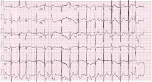
Figure 1:Señal de electrocardiograma.

Figure 2:Señal de audio.
La formalización de la respuesta al impulso de los sistemas LTI ha proporcionado una herramienta de gran utilidad, ya que una única señal, la respuesta al impulso del sistema, permite predecir su comportamiento ante cualquier señal de entrada y, en último término, caracterizar propiedades fundamentales como la estabilidad, la causalidad o la presencia de memoria.
No obstante, la caracterización de señales y sistemas en el dominio temporal se basa en una operación relativamente compleja como es la convolución, lo que dificulta tanto la interpretación cualitativa de la transformación que lleva a cabo un sistema LTI como la predicción directa de la forma de la señal de salida ante una entrada dada.

Figure 3:Diagrama de bloques de un sistema: y(t)=T{x(t)}.
En el presente tema se introduce una caracterización alternativa en el dominio espectral, o dominio de la frecuencia para señales en tiempo continuo. La ventaja de esta representación es doble:
Por un lado, la descripción de las señales y los sistemas en términos de su contenido frecuencial conecta de forma natural con fenómenos físicos cotidianos.
Por otro lado, el efecto de un sistema LTI sobre una señal de entrada se describe en términos de una operación mucho más sencilla que la convolución con la respuesta al impulso h(t): la relación entrada-salida se reduce al producto por una respuesta en frecuencia H(ω).
Ejemplo 1: El tono de las notas musicales
La diferencia entre dos notas musicales de una misma octava está asociada a su frecuencia o armónico fundamental.
import numpy as np
from bokeh.plotting import figure, show, output_notebook
from bokeh.models import ColumnDataSource, CustomJS, TapTool, HoverTool, LabelSet, Div, RadioButtonGroup
from bokeh.layouts import column, row

# Configuración silenciosa
output_notebook(verbose=False, hide_banner=True)

# ==========================================
# 1. DEFINICIÓN DE DATOS
# ==========================================
notes_data = [
    {'note': 'Do (C4)', 'freq': 261.63, 'x': 1, 'w': 1, 'h': 4, 'type': 'w'},
    {'note': 'Do# (C#4) / Re♭ (D♭4)', 'freq': 277.18, 'x': 1.5, 'w': 0.6, 'h': 2.5, 'type': 'b'},
    {'note': 'Re (D4)', 'freq': 293.66, 'x': 2, 'w': 1, 'h': 4, 'type': 'w'},
    {'note': 'Re# (D#4) / Mi♭ (E♭4)', 'freq': 311.13, 'x': 2.5, 'w': 0.6, 'h': 2.5, 'type': 'b'},
    {'note': 'Mi (E4)', 'freq': 329.63, 'x': 3, 'w': 1, 'h': 4, 'type': 'w'},
    {'note': 'Fa (F4)', 'freq': 349.23, 'x': 4, 'w': 1, 'h': 4, 'type': 'w'},
    {'note': 'Fa# (F#4) / Sol♭ (G♭4)', 'freq': 369.99, 'x': 4.5, 'w': 0.6, 'h': 2.5, 'type': 'b'},
    {'note': 'Sol (G4)', 'freq': 392.00, 'x': 5, 'w': 1, 'h': 4, 'type': 'w'},
    {'note': 'Sol# (G#4) / La♭ (A♭4)', 'freq': 415.30, 'x': 5.5, 'w': 0.6, 'h': 2.5, 'type': 'b'},
    {'note': 'La (A4)', 'freq': 440.00, 'x': 6, 'w': 1, 'h': 4, 'type': 'w'},
    {'note': 'La# (A#4) / Si♭ (B♭4)', 'freq': 466.16, 'x': 6.5, 'w': 0.6, 'h': 2.5, 'type': 'b'},
    {'note': 'Si (B4)', 'freq': 493.88, 'x': 7, 'w': 1, 'h': 4, 'type': 'w'},
]

whites = [n for n in notes_data if n['type'] == 'w']
blacks = [n for n in notes_data if n['type'] == 'b']

source_white = ColumnDataSource(data=dict(
    x=[k['x'] for k in whites], y=[k['h']/2 for k in whites],
    width=[k['w'] for k in whites], height=[k['h'] for k in whites],
    note_name=[k['note'] for k in whites], freq_val=[k['freq'] for k in whites],
    color=['white'] * len(whites)
))

source_black = ColumnDataSource(data=dict(
    x=[k['x'] for k in blacks], y=[k['h']/2 for k in blacks],
    width=[k['w'] for k in blacks], height=[k['h'] for k in blacks],
    note_name=[k['note'] for k in blacks], freq_val=[k['freq'] for k in blacks],
    color=['black'] * len(blacks)
))

# Datos Señales
initial_freq = 261.63
source_spectrum = ColumnDataSource(data=dict(freqs=[initial_freq], amps=[1.0], zeros=[0.0], labels=[f"{initial_freq} Hz"]))
t_max = 0.02
t_vec = np.linspace(0, t_max, 500)
y_vec = np.sin(2 * np.pi * initial_freq * t_vec)
source_time = ColumnDataSource(data=dict(t=t_vec, y=y_vec))


# ==========================================
# NUEVO WIDGET: CONTROL DE SONIDO
# ==========================================
sound_control = RadioButtonGroup(labels=["Silencio 🔇", "Sonido Activado 🔊"], active=0)


# ==========================================
# FIGURAS
# ==========================================

# 1. TECLADO
p_keys = figure(height=220, tools="tap", sizing_mode="stretch_width",
                title="1. Haz clic en una tecla",
                y_range=(4.2, -0.2))
p_keys.toolbar_location = None
p_keys.axis.visible = False
p_keys.grid.visible = False
p_keys.outline_line_color = None

renderer_w = p_keys.rect(x='x', y='y', width='width', height='height',
                         fill_color='color', line_color="gray", source=source_white)
renderer_b = p_keys.rect(x='x', y='y', width='width', height='height',
                         fill_color='color', line_color="gray", source=source_black)

renderer_w.selection_glyph = renderer_w.glyph.clone()
renderer_w.selection_glyph.fill_color = "#ADD8E6"
renderer_w.nonselection_glyph = renderer_w.glyph
renderer_b.selection_glyph = renderer_b.glyph.clone()
renderer_b.selection_glyph.fill_color = "#ADD8E6"
renderer_b.nonselection_glyph = renderer_b.glyph

tap_tool = p_keys.select(type=TapTool)
p_keys.add_tools(HoverTool(renderers=[renderer_w, renderer_b], tooltips=[("Nota", "@note_name"), ("Frec.", "@freq_val Hz")]))

# 2. TIEMPO
p_time = figure(height=300, title=f"2. Dominio del Tiempo (x(t))", sizing_mode="stretch_width",
                x_axis_label="Tiempo (s)", y_axis_label="Amplitud",
                y_range=(-1.2, 1.2), x_range=(0, t_max))
p_time.line(x='t', y='y', line_width=2, color="#1f77b4", source=source_time)

# 3. FRECUENCIA
p_spec = figure(height=300, title="3. Dominio de la Frecuencia (|X(f)|)", sizing_mode="stretch_width",
                x_axis_label="Frecuencia (Hz)", y_axis_label="Magnitud",
                x_range=(200, 550), y_range=(0, 1.3))
p_spec.segment(x0='freqs', y0='zeros', x1='freqs', y1='amps', line_width=3, color="#d62728", source=source_spectrum)
p_spec.scatter(x='freqs', y='amps', size=10, color="#d62728", fill_color="white", source=source_spectrum)
labels = LabelSet(x='freqs', y='amps', text='labels', level='glyph', x_offset=5, y_offset=5, source=source_spectrum,
                  text_font_size="10pt", text_color="#d62728")
p_spec.add_layout(labels)

# ==========================================
# INTERACTIVIDAD (JS con AUDIO)
# ==========================================
callback = CustomJS(args=dict(source_w=source_white, source_b=source_black,
                              source_spec=source_spectrum, source_time=source_time,
                              p_spec=p_spec, p_time=p_time,
                              sound_control=sound_control), code="""
    const idx_b = source_b.selected.indices;
    const idx_w = source_w.selected.indices;
    let new_freq = null;
    let new_note = "";

    // 1. Detectar tecla
    if (idx_b.length > 0) {
        const i = idx_b[0];
        new_freq = source_b.data['freq_val'][i];
        new_note = source_b.data['note_name'][i];
        source_w.selected.indices = [];
    } else if (idx_w.length > 0) {
        const i = idx_w[0];
        new_freq = source_w.data['freq_val'][i];
        new_note = source_w.data['note_name'][i];
    }

    if (new_freq !== null) {
        // 2. Actualizar Gráficas
        source_spec.data['freqs'] = [new_freq];
        source_spec.data['labels'] = [new_freq.toFixed(2) + " Hz"];
        p_spec.title.text = "Frecuencia: " + new_freq.toFixed(1) + " Hz (" + new_note + ")";
        source_spec.change.emit();

        const t = source_time.data['t'];
        const y = source_time.data['y'];
        const omega = 2 * Math.PI * new_freq;
        for (let k = 0; k < t.length; k++) { y[k] = Math.sin(omega * t[k]); }
        p_time.title.text = "Tiempo: " + new_note;
        source_time.change.emit();

        // 3. GENERACIÓN DE SONIDO (Piano Attack)
        // Comprobamos si el radio button está en "Sonido Activado" (índice 1)
        if (sound_control.active === 1) {

            // Inicializar AudioContext (Singleton)
            if (!window.audioCtx) {
                window.audioCtx = new (window.AudioContext || window.webkitAudioContext)();
            }
            const ctx = window.audioCtx;
            if (ctx.state === 'suspended') { ctx.resume(); }

            const now = ctx.currentTime;

            // Oscilador (Seno puro, consistente con la gráfica)
            const osc = ctx.createOscillator();
            const gain = ctx.createGain();

            osc.frequency.value = new_freq;
            osc.type = 'sine';

            // --- ENVOLVENTE TIPO PIANO (Exponential Decay) ---
            // 1. Silencio inicial
            gain.gain.setValueAtTime(0, now);

            // 2. Ataque percusivo (muy rápido, 0.02s) hasta volumen medio
            gain.gain.linearRampToValueAtTime(0.5, now + 0.02);

            // 3. Decaimiento natural (Exponential Release)
            // Simula la cuerda perdiendo energía libremente
            gain.gain.exponentialRampToValueAtTime(0.001, now + 1.5);

            // Conectar y reproducir
            osc.connect(gain);
            gain.connect(ctx.destination);

            osc.start(now);
            osc.stop(now + 1.5); // Detener oscilador cuando el sonido ya es inaudible
        }
    }
""")
tap_tool.callback = callback

# ==========================================
# CAPTION Y LAYOUT
# ==========================================
texto_caption = """
<div style="font-family: sans-serif; margin-top: 10px; font-size: 14px; opacity: 0.8;">
    <b>Ejemplo 1: Notas musicales.</b> Activa el sonido con el botón superior y pulsa las teclas.
    Observa cómo varía el periodo fundamental de la señal en el tiempo (azul),
    y en frecuencia varía la posición de la frecuencia fundamental (rojo).<br>
    <b>Nota:</b> La señal visualizada es una onda pura (modo fundamental), mientras que el sonido simula
    el ataque percusivo de un piano aplicando una envolvente de amplitud exponencial.
</div>
"""
caption = Div(text=texto_caption, sizing_mode="stretch_width")

# Añadimos el control de sonido al layout
layout = column(sound_control, p_keys, row(p_time, p_spec, sizing_mode="stretch_width"), caption, sizing_mode="scale_width")

show(layout)Ejemplo 2: el timbre de los instrumentos musicales
El timbre de un instrumento viene determinado por la distinta combinación de armónicos que lo componen.
El instrumento o su caja de resonancia son un sistema LTI que modifica la señal de entrada, que es el sonido (fundamental con armónicos de frecuencias múltiplos de la fundamental) generado al pulsar una cuerda o producir una onda dentro del tubo.
Por tanto, tendrá su respuesta al impulso, que en frecuencia (su respuesta en frecuencia) modifica la contribución de cada uno de los armónicos originados dentro del intrumento.
import numpy as np
import json
from bokeh.plotting import figure, show, output_notebook
from bokeh.models import ColumnDataSource, CustomJS, Select, HoverTool, Div, Button
from bokeh.layouts import column, row

output_notebook(verbose=False, hide_banner=True)

# ==========================================
# 1. PARÁMETROS Y DATOS
# ==========================================
MAX_FREQ_VIEW = 3000
N_HARMONICS = 25

def extend_profile(base_profile, length):
    res = list(base_profile)
    if len(res) < length:
        res += [0.0] * (length - len(res))
    return res[:length]

violin_profile = []
for i in range(1, N_HARMONICS + 1):
    val = 1.0 / i
    if i > 4: val = val * 0.5
    violin_profile.append(val)

instruments = {
    "Tono Puro": extend_profile([1.0], N_HARMONICS),
    "Clarinete": extend_profile([1.0, 0.1, 0.8, 0.05, 0.6, 0.02, 0.4, 0, 0.2, 0, 0.1], N_HARMONICS),
    "Trompeta":  extend_profile([0.8, 1.0, 0.7, 0.9, 0.5, 0.7, 0.4, 0.5, 0.3, 0.2, 0.15, 0.1, 0.05], N_HARMONICS),
    "Flauta":    extend_profile([1.0, 0.4, 0.1, 0.05, 0.02, 0.01], N_HARMONICS),
    "Violín":    violin_profile,
    "Sierra":    [1.0/(i+1) for i in range(N_HARMONICS)],
    "Cuadrada":  [1.0/(i+1) if (i+1)%2!=0 else 0 for i in range(N_HARMONICS)]
}

notes_map = {
    "Do grave (C3)": 130.81,
    "La (A3)": 220.00,
    "Do central (C4)": 261.63,
    "Mi (E4)": 329.63,
    "La (A4)": 440.00,
    "Do agudo (C5)": 523.25
}

instruments_json = json.dumps(instruments)
notes_json = json.dumps(notes_map)

init_inst = "Violín"
init_note = "La (A3)"
init_amps = instruments[init_inst]
f0 = notes_map[init_note]
indices = np.arange(1, N_HARMONICS + 1)

# CDS Frecuencia
freqs_init = indices * f0
source_freq = ColumnDataSource(data=dict(
    h_idx=indices, freq=freqs_init, amp=init_amps, zeros=np.zeros(N_HARMONICS)
))

# CDS Tiempo
t_vec = np.linspace(0, 0.02, 800)
y_init = np.zeros_like(t_vec)
for i, amp in enumerate(init_amps):
    if amp > 0: y_init += amp * np.sin(2 * np.pi * (i+1) * f0 * t_vec)
if np.max(np.abs(y_init)) > 0: y_init /= np.max(np.abs(y_init))

source_time = ColumnDataSource(data=dict(t=t_vec, y=y_init))

# ==========================================
# 2. INTERFAZ GRÁFICA
# ==========================================
select_inst = Select(title="Timbre:", value=init_inst, options=list(instruments.keys()), width=200)
select_note = Select(title="Nota:", value=init_note, options=list(notes_map.keys()), width=200)
button_play = Button(label="▶ Escuchar", button_type="success", width=200, height=50)

# Gráfico TIEMPO
p_time = figure(height=300, title="Dominio del Tiempo (20 ms)", sizing_mode="stretch_width",
                x_axis_label="Tiempo (s)", y_axis_label="Amplitud Normalizada",
                y_range=(-1.3, 1.3), x_range=(0, 0.02))
p_time.line(x='t', y='y', line_width=2, color="#1f77b4", source=source_time)
p_time.grid.grid_line_alpha = 0.3

# Gráfico FRECUENCIA
p_freq = figure(height=300, title=f"Espectro (límite {MAX_FREQ_VIEW} Hz)", sizing_mode="stretch_width",
                x_axis_label="Frecuencia (Hz)", y_axis_label="Amplitud Relativa",
                x_range=(0, MAX_FREQ_VIEW), y_range=(0, 1.2))

# Deltas (Stems)
p_freq.segment(x0='freq', y0='zeros', x1='freq', y1='amp', line_width=3, color="#d62728", source=source_freq)
# Cabezas (Puntos)
p_freq.scatter(x='freq', y='amp', size=8, color="#d62728", fill_color="white", line_width=2, source=source_freq)

# --- ELIMINADA LA LÍNEA PUNTEADA (ENVOLVENTE) ---
# p_freq.line(...)  <-- Eliminado para evitar confusión visual

p_freq.add_tools(HoverTool(tooltips=[("n", "@h_idx"), ("f", "@freq{0.} Hz"), ("Amp", "@amp{0.00}")], mode='vline'))

# ==========================================
# 3. LÓGICA DE ACTUALIZACIÓN (JS)
# ==========================================
js_update_code = """
    const inst_name = select_inst.value;
    const note_name = select_note.value;
    const instruments_db = JSON.parse(inst_json_str);
    const notes_db = JSON.parse(notes_json_str);

    const new_amps = instruments_db[inst_name];
    const f0 = notes_db[note_name];

    if (!new_amps || !f0) return;

    // Update Frecuencia
    const freqs_array = source_freq.data['freq'];
    const amps_array = source_freq.data['amp'];

    for (let i = 0; i < N; i++) {
        freqs_array[i] = (i + 1) * f0;
        amps_array[i] = new_amps[i];
    }
    source_freq.change.emit();

    // Update Tiempo
    const t = source_time.data['t'];
    const y = source_time.data['y'];
    const omega0 = 2 * Math.PI * f0;

    let max_val = 0;
    for (let i = 0; i < t.length; i++) {
        let sum = 0;
        for (let h = 0; h < N; h++) {
             const amp = new_amps[h];
             if (amp > 0) sum += amp * Math.sin((h + 1) * omega0 * t[i]);
        }
        y[i] = sum;
        if (Math.abs(sum) > max_val) max_val = Math.abs(sum);
    }
    if (max_val > 0.0001) { for (let i = 0; i < t.length; i++) { y[i] = y[i] / max_val; } }
    source_time.change.emit();
"""

callback_update = CustomJS(args=dict(source_freq=source_freq, source_time=source_time,
                              select_inst=select_inst, select_note=select_note,
                              N=N_HARMONICS, inst_json_str=instruments_json, notes_json_str=notes_json),
                    code=js_update_code)

select_inst.js_on_change('value', callback_update)
select_note.js_on_change('value', callback_update)

# ==========================================
# 4. AUDIO (NORMALIZADO + ENVOLVENTE)
# ==========================================
js_play_code = """
    if (!window.audioCtx) { window.audioCtx = new (window.AudioContext || window.webkitAudioContext)(); }
    const ctx = window.audioCtx;
    if (ctx.state === 'suspended') { ctx.resume(); }

    const freqs = source_freq.data['freq'];
    const amps = source_freq.data['amp'];

    // Normalización para evitar saturación
    let totalAmp = 0;
    for (let i = 0; i < amps.length; i++) totalAmp += amps[i];
    const scaleFactor = (totalAmp > 0) ? (0.9 / totalAmp) : 0;

    const now = ctx.currentTime;
    const attackTime = 0.15;
    const holdTime = 1.0;
    const releaseTime = 0.5;
    const totalDuration = attackTime + holdTime + releaseTime;

    const masterGain = ctx.createGain();
    masterGain.gain.setValueAtTime(0, now);
    masterGain.gain.linearRampToValueAtTime(0.5, now + attackTime);
    masterGain.gain.setValueAtTime(0.5, now + attackTime + holdTime);
    masterGain.gain.linearRampToValueAtTime(0, now + totalDuration);
    masterGain.connect(ctx.destination);

    for (let i = 0; i < freqs.length; i++) {
        const rawAmp = amps[i];
        if (rawAmp > 0.001) {
            const osc = ctx.createOscillator();
            const gain = ctx.createGain();
            osc.frequency.value = freqs[i];
            osc.type = 'sine';
            gain.gain.value = rawAmp * scaleFactor;
            osc.connect(gain);
            gain.connect(masterGain);
            osc.start(now);
            osc.stop(now + totalDuration);
        }
    }
"""

callback_play = CustomJS(args=dict(source_freq=source_freq), code=js_play_code)
button_play.js_on_event('button_click', callback_play)

# ==========================================
# 5. LAYOUT FINAL
# ==========================================
texto_caption = """
<div style="font-family: sans-serif; margin-top: 10px; font-size: 13px; opacity: 0.8;">
    <b>Ejemplo 2: Timbre de distintos instrumentos.</b> Seleccionando un instrumento y una nota, observa cómo cambia
    la señal en el tiempo y su espectro armónico. Cada instrumento (su respuesta al impulso) tiene distinta contribución
    de armónicos, lo que afecta al color del sonido.
</div>
"""
caption = Div(text=texto_caption, sizing_mode="stretch_width")

widgets_row = row(select_inst, select_note, button_play)
layout = column(widgets_row, row(p_time, p_freq, sizing_mode="stretch_width"), caption, sizing_mode="scale_width")

show(layout)Ejemplo 3: Receptor de radio
La coexistencia de múltiples emisoras de radio en un mismo medio físico es posible gracias a la modulación de cada señal en torno a una frecuencia portadora distinta.
import numpy as np
import json
from bokeh.plotting import figure, show, output_notebook
from bokeh.models import ColumnDataSource, CustomJS, Slider, Div, Button
from bokeh.layouts import column, row

output_notebook(verbose=False, hide_banner=True)

# ==========================================
# 1. PARÁMETROS
# ==========================================
NOISE_LEVEL = 0.8
freq_min, freq_max = 87.5, 108.0
filter_width = 0.6
bw_station = 0.7

# ==========================================
# 2. DATOS
# ==========================================
melody_rock = [164.8, 164.8, 196.0, 164.8, 146.8, 130.8, 110.0, 110.0]
# Himno de la Alegría (Ode to Joy)
# Mi, Mi, Fa, Sol, Sol, Fa, Mi, Re, Do, Do, Re, Mi, Mi, Re, Re
melody_classic = [
    329.6, 329.6, 349.2, 392.0,
    392.0, 349.2, 329.6, 293.7,
    261.6, 261.6, 293.7, 329.6,
    329.6, 293.7, 293.7
]
melody_pop  = [261.6, 261.6, 293.7, 329.6, 261.6, 329.6, 293.7, 261.6]
melody_scifi = [440, 880, 660, 440, 220, 880, 440, 660]

stations = [
    {"freq": 90.2,  "bw": bw_station, "name": "Rock FM (90.0)", "type": "sq", "melody": melody_rock},
    {"freq": 93.1,  "bw": bw_station, "name": "Música Clásica (93.1)", "type": "sin", "melody": melody_classic},
    {"freq": 94.5, "bw": bw_station, "name": "Pop Hits (94.5)", "type": "saw", "melody": melody_pop},
    {"freq": 100.4, "bw": bw_station, "name": "Cyber Hz (100.4)", "type": "saw", "melody": melody_scifi}
]

# Espectro Estático
x_spec = np.linspace(freq_min, freq_max, 1000)
noise_scale = 0.02 + (NOISE_LEVEL * 0.4)
noise_floor = np.random.normal(noise_scale, noise_scale/3, size=len(x_spec))
y_spec_total = np.abs(noise_floor)

for st in stations:
    y_s = 0.9 * np.exp(-0.5 * ((x_spec - st["freq"]) / (st["bw"]/2.0))**2)
    y_spec_total += y_s

source_spectrum = ColumnDataSource(data=dict(x=np.concatenate([[x_spec[0]], x_spec, [x_spec[-1]]]), y=np.concatenate([[0], y_spec_total, [0]])))

# Filtro
center_init = 88.0
x_filt_box = [center_init - filter_width, center_init - filter_width, center_init + filter_width, center_init + filter_width]
y_filt_box = [0, 1.3, 1.3, 0]
source_filter_box = ColumnDataSource(data=dict(x=x_filt_box, y=y_filt_box))

# Filtrado
y_filtered = np.zeros_like(x_spec)
source_filtered_spec = ColumnDataSource(data=dict(x=np.concatenate([[x_spec[0]], x_spec, [x_spec[-1]]]), y=np.concatenate([[0], y_filtered, [0]])))

# Tiempo
t_vec = np.linspace(0, 0.05, 400)
y_time = np.random.rand(400) - 0.5
source_time = ColumnDataSource(data=dict(t=t_vec, y=y_time))

# JSONs
stations_json = json.dumps(stations)
x_spec_json = json.dumps(x_spec.tolist())
y_total_json = json.dumps(y_spec_total.tolist())

# ==========================================
# 3. INTERFAZ
# ==========================================
CONTROL_WIDTH = 280

lcd_html = """
<div style="background-color: #111; color: #ff3333; font-family: 'Courier New', monospace; font-weight: bold; font-size: 24px; text-align: center; border: 4px solid #444; border-radius: 8px; padding: 10px; margin-bottom: 20px;">
    <div style="font-size: 12px; color: #555; margin-bottom:5px; display:flex; justify-content:space-between;">
        <span>SIGNAL</span><span id="tuned_led" style="color:#330000">● LOCKED</span>
    </div>
    <span id='freq_val' style="font-size:32px;">88.0</span> MHz
</div>
"""
div_lcd = Div(text=lcd_html, width=CONTROL_WIDTH)
slider_tuner = Slider(start=freq_min, end=freq_max, value=88.0, step=0.05, title="DIAL FM", width=CONTROL_WIDTH)

# BOTÓN CON ID EXPLÍCITO PARA REFERENCIA
toggle_audio = Button(label="🔇 ENCENDER RADIO", button_type="danger", width=CONTROL_WIDTH)

# GRÁFICAS
p_in = figure(height=180, title="1. Banda FM (Entrada Antena)", sizing_mode="stretch_width",
              x_axis_label="Frecuencia (MHz)", y_axis_label="Amp", x_range=(freq_min, freq_max), y_range=(0, 1.4), tools="")
p_in.background_fill_color = "#111"
p_in.patch(x='x', y='y', color="#39ff14", alpha=0.3, source=source_spectrum)
p_in.line(x='x', y='y', color="#ff9900", line_width=2, alpha=0.8, source=source_filter_box)
p_in.patch(x='x', y='y', color="#ff9900", alpha=0.1, source=source_filter_box)

p_mid = figure(height=160, title="2. Selección (Paso Banda)", sizing_mode="stretch_width",
               x_axis_label="Frecuencia (MHz)", y_axis_label="Amp", x_range=(freq_min, freq_max), y_range=(0, 1.4), tools="")
p_mid.background_fill_color = "#111"
p_mid.patch(x='x', y='y', color="#00ffff", alpha=0.6, line_width=2, line_color="#00ffff", source=source_filtered_spec)

p_out = figure(height=160, title="3. Señal Demodulada (Audio)", sizing_mode="stretch_width",
               x_axis_label="Tiempo (s)", y_axis_label="Voltaje", y_range=(-1.5, 1.5), tools="")
p_out.background_fill_color = "#222"
p_out.line(x='t', y='y', line_width=2, color="#ecf0f1", source=source_time)


# ==========================================
# 4. LÓGICA VISUAL
# ==========================================
js_tuner_code = """
    const f_center = slider.value;
    const width = filter_w;

    // Display
    let new_html = div_lcd.text.replace(/>[0-9]+\.[0-9]</, ">" + f_center.toFixed(1) + "<");

    // Filtro
    const x_box = source_box.data['x'];
    x_box[0] = f_center - width; x_box[1] = f_center - width;
    x_box[2] = f_center + width; x_box[3] = f_center + width;
    source_box.change.emit();

    // Espectro
    const x_arr = JSON.parse(x_json);
    const y_total_arr = JSON.parse(y_json);
    const y_filt_plot = source_filt_spec.data['y'];
    const f_start = f_center - width;
    const f_end = f_center + width;
    for (let i = 0; i < x_arr.length; i++) {
        const f = x_arr[i];
        if (f >= f_start && f <= f_end) y_filt_plot[i+1] = y_total_arr[i];
        else y_filt_plot[i+1] = 0;
    }
    source_filt_spec.change.emit();

    // Lock Logic
    const stations = JSON.parse(st_json);
    let best_station = -1;
    let min_dist = 999;
    for(let i=0; i<stations.length; i++){
        const dist = Math.abs(f_center - stations[i].freq);
        if(dist < min_dist){ min_dist = dist; best_station = i; }
    }
    const lock_range = 0.3;
    const fade_range = 1.5;
    let is_locked = false;
    let signal_strength = 0;
    if (min_dist <= lock_range) { is_locked = true; signal_strength = 1.0; }
    else if (min_dist < fade_range) { signal_strength = 1.0 - ((min_dist - lock_range) / (fade_range - lock_range)); }

    if (is_locked) new_html = new_html.replace(/color:#[0-9a-fA-F]+">● LOCKED/, 'color:#00ff00">● LOCKED');
    else new_html = new_html.replace(/color:#[0-9a-fA-F]+">● LOCKED/, 'color:#330000">● LOCKED');
    div_lcd.text = new_html;

    window.radioState = { strength: signal_strength, stationIdx: best_station, locked: is_locked };

    // Wave Visual
    const t = source_time.data['t'];
    const y = source_time.data['y'];
    let vis_freq = 50 + (best_station * 80);
    for (let i = 0; i < t.length; i++) {
        if (is_locked) {
            y[i] = Math.sin(2 * Math.PI * vis_freq * t[i]) * (1 + 0.3*Math.sin(25*t[i]));
        } else {
            const noise = (Math.random() * 2) - 1;
            let signal = 0;
            if (signal_strength > 0.01) signal = Math.sin(2 * Math.PI * vis_freq * t[i]);
            y[i] = (noise * (1-signal_strength)) + (signal * signal_strength);
        }
    }
    source_time.change.emit();

    if (window.updateRadioVol) window.updateRadioVol();
"""

callback_tuner = CustomJS(args=dict(source_box=source_filter_box, source_filt_spec=source_filtered_spec,
    source_time=source_time, slider=slider_tuner, div_lcd=div_lcd, st_json=stations_json,
    x_json=x_spec_json, y_json=y_total_json, filter_w=filter_width), code=js_tuner_code)
slider_tuner.js_on_change('value', callback_tuner)

# ==========================================
# 5. AUDIO ENGINE (FIXED BUTTON LOGIC)
# ==========================================
js_audio_init = """
    // Usamos 'btn_obj' pasado en args para asegurar la referencia correcta
    const btn = btn_obj;
    const stations = JSON.parse(st_json);
    const MAX_NOISE = noise_vol;

    // --- LÓGICA DE ESTADO DEL BOTÓN ---
    if (window.isRadioOn) {
        // --- APAGAR ---
        window.isRadioOn = false;

        // 1. Cambiar aspecto visual INMEDIATAMENTE
        btn.label = "🔇 ENCENDER RADIO";
        btn.button_type = "danger";

        // 2. Detener Audio
        if (window.currentAudioCtx) window.currentAudioCtx.suspend();
        if (window.melodyInterval) clearInterval(window.melodyInterval);
        return;
    }

    // --- ENCENDER ---
    window.isRadioOn = true;

    // 1. Cambiar aspecto visual INMEDIATAMENTE
    btn.label = "🔊 APAGAR RADIO";
    btn.button_type = "success";

    // 2. Inicializar Contexto
    if (!window.currentAudioCtx) window.currentAudioCtx = new (window.AudioContext || window.webkitAudioContext)();
    const ctx = window.currentAudioCtx;
    if (ctx.state === 'suspended') ctx.resume();

    // 3. Crear Nodos de Audio
    // -- Ruido --
    if (!window.noiseGainNode) {
        const bSize = ctx.sampleRate * 2;
        const buffer = ctx.createBuffer(1, bSize, ctx.sampleRate);
        const data = buffer.getChannelData(0);
        for (let i = 0; i < bSize; i++) data[i] = (Math.random() * 2 - 1) * MAX_NOISE;
        const nSource = ctx.createBufferSource(); nSource.buffer = buffer; nSource.loop = true;
        const nFilter = ctx.createBiquadFilter(); nFilter.type = 'lowpass'; nFilter.frequency.value = 500;
        const nGain = ctx.createGain(); nGain.gain.setValueAtTime(MAX_NOISE, ctx.currentTime);
        nSource.connect(nFilter); nFilter.connect(nGain); nGain.connect(ctx.destination); nSource.start();
        window.noiseGainNode = nGain;
    }
    // -- Osciladores --
    if (!window.oscNodes) {
        window.oscNodes = [];
        for(let i=0; i<stations.length; i++){
            const osc = ctx.createOscillator();
            const gain = ctx.createGain();
            if (stations[i].type === 'sq') osc.type = 'square';
            else if (stations[i].type === 'saw') osc.type = 'sawtooth';
            else osc.type = 'sine';
            osc.frequency.value = 440; gain.gain.setValueAtTime(0, ctx.currentTime);
            osc.connect(gain); gain.connect(ctx.destination); osc.start();
            window.oscNodes.push({osc: osc, gain: gain});
        }
    }
    // -- Secuenciador --
    if (window.melodyInterval) clearInterval(window.melodyInterval);
    let noteStep = 0;
    window.melodyInterval = setInterval(() => {
        noteStep++;
        for(let i=0; i<stations.length; i++){
            const melody = stations[i].melody;
            window.oscNodes[i].osc.frequency.setValueAtTime(melody[noteStep % melody.length], ctx.currentTime);
        }
    }, 200);

    // 4. Activar Mixer loop
    window.updateRadioVol = function() {
        if (!window.radioState || !window.isRadioOn) return;

        const is_locked = window.radioState.locked;
        const s = window.radioState.strength;
        const best = window.radioState.stationIdx;
        const now = ctx.currentTime;

        if (is_locked) {
            window.noiseGainNode.gain.cancelScheduledValues(now);
            window.noiseGainNode.gain.setValueAtTime(0, now);
            for(let i=0; i<stations.length; i++){
                const vol = (i === best) ? 0.3 : 0;
                window.oscNodes[i].gain.gain.setTargetAtTime(vol, now, 0.1);
            }
        } else {
            let noiseLvl = MAX_NOISE * (1 - s);
            window.noiseGainNode.gain.setTargetAtTime(noiseLvl, now, 0.1);
            for(let i=0; i<stations.length; i++){
                let musicLvl = (i === best) ? (0.3 * s) : 0;
                window.oscNodes[i].gain.gain.setTargetAtTime(musicLvl, now, 0.1);
            }
        }
    };

    // Forzar un update inicial
    slider.value = slider.value;
"""

# PASAMOS EL BOTÓN EXPLÍCITAMENTE EN LOS ARGUMENTOS 'btn_obj'
toggle_audio.js_on_event('button_click', CustomJS(args=dict(st_json=stations_json, slider=slider_tuner, noise_vol=NOISE_LEVEL, btn_obj=toggle_audio), code=js_audio_init))

# ==========================================
# 6. LAYOUT FINAL
# ==========================================
controls_col = column(div_lcd, slider_tuner, toggle_audio)

desc = Div(text="""
<div style='width:280px; color:#aaa; font-family:sans-serif; margin-top:20px;'>
    <b>Radio FM:</b>
    <br>Sintoniza: <b>90.2, 93.1, 94.5, 100.4 MHz</b>.
    <br><br>
    Nota cómo al multiplicar la respuesta en frecuencia del sistema (naranja) por la señal de entrada, se sintoniza cada una de las emisiones indidivuales.
</div>""", width=CONTROL_WIDTH)

texto_caption = """
<div style="font-family: sans-serif; margin-top: 10px; font-size: 13px; opacity: 0.8;">
    <b>Receptor de radio:</b><br>
    El receptor simula la sintonización de varias emisoras de radio FM transmitidas a distintas frecuencias del espectro radioeléctrico.
    Mueve el dial para sintonizar las distintas emisoras y escuchar su melodía característica.
</div>
"""
caption = Div(text=texto_caption, sizing_mode="stretch_width")

plots_col = column(p_in, p_mid, p_out, sizing_mode="stretch_width")
layout = row(column(controls_col, desc), plots_col, sizing_mode="stretch_width")
layout2 = column(layout, caption, sizing_mode="scale_width")
layout.background = "#000"

show(layout2)Ejemplo 4: Modelo fuente-filtro del habla
El habla se puede modelar como la salida de un sistema lineal. La entrada es la vibración de las cuerdas vocales (periódica) o el aire turbulento (ruido), y el sistema es el tracto vocal (boca y garganta), que modifica esta señal. Dado que movemos la boca al hablar, la respuesta al impulso del sistema es variante en el tiempo; sin embargo, para cada fonema individual, podemos analizarlo como un sistema LTI fijo (mientras no cambiemos la articulación).
En el dominio de la frecuencia, este sistema introduce picos de resonancia llamados formantes: el primero (F1) depende de la apertura de la boca (frecuencias inferiores a 1000 Hz) y el segundo (F2) de la posición de la lengua.
En la gráfica interactiva inferior se descompone la palabra ‘Eso’. Se puede ver claramente la diferencia entre la entrada periódica de las vocales —cuyos armónicos se ven amplificados por los formantes— y la naturaleza ruidosa y aperiódica de la ‘s’, generada por la fricción del aire contra los dientes.
import numpy as np
import librosa
import scipy.signal
import base64
import io
import os
from scipy.io.wavfile import write as wav_write
from bokeh.plotting import figure, show, output_notebook
from bokeh.models import ColumnDataSource, CustomJS, Select, BoxAnnotation, Range1d, Slider, Div
from bokeh.layouts import column, row

output_notebook()

# ==============================================================================
#  CONFIGURACIÓN GLOBAL (VARIABLES DE CONTROL)
# ==============================================================================
FILENAME = 'figures/T3/mi_voz.mp3'
ZCR_THRESHOLD = 0.08      # Umbral ajustado según tu feedback
N_FFT = 1024*4              # Resolución de la FFT (Puntos)
MODO_LOGARITMICO = True  # True = dB (Log), False = Lineal Normalizada (Natural)
FREQ_MAX_VISUAL = 5000    # Límite del eje X en Hz (5000 Hz es estándar para voz)

# ==============================================================================
# 1. CARGA Y PREPROCESADO
# ==============================================================================
# Comprobación de seguridad por si el archivo no existe en esa ruta
if not os.path.exists(FILENAME):
    print(f"ADVERTENCIA: No se encuentra '{FILENAME}'. Usando audio dummy o ruta local.")
    # Si tienes el archivo en la misma carpeta, descomenta esto:
    # FILENAME = "mi_voz.mp3"

y_raw, sr = librosa.load(FILENAME, sr=None)
y_trimmed, _ = librosa.effects.trim(y_raw, top_db=20)
duration = len(y_trimmed) / sr
time_axis = np.linspace(0, duration, len(y_trimmed))

# ==============================================================================
# 2. SEGMENTACIÓN INTELIGENTE
# ==============================================================================
zcr = librosa.feature.zero_crossing_rate(y_trimmed, frame_length=2048, hop_length=512)[0]
times_zcr = librosa.frames_to_samples(range(len(zcr)), hop_length=512) / sr
is_fricative = zcr > ZCR_THRESHOLD

s_indices = np.where(is_fricative)[0]
cuts = {}

if len(s_indices) > 0:
    t_start_s = max(0, min(times_zcr[s_indices[0]], duration))
    t_end_s   = max(0, min(times_zcr[s_indices[-1]], duration))
    cuts["e (Vocal)"]     = (0.0, t_start_s)
    cuts["s (Fricativa)"] = (t_start_s, t_end_s)
    cuts["a (Vocal)"]     = (t_end_s, duration)
else:
    # Fallback si no detecta la S
    cuts = {"Inicio": (0, duration/3), "Medio": (duration/3, 2*duration/3), "Final": (2*duration/3, duration)}

# ==============================================================================
# 3. ANÁLISIS
# ==============================================================================
def analyze_segment(y_in, sr, t_start, t_end, name):
    idx_start = max(0, int(t_start * sr))
    idx_end = min(len(y_in), int(t_end * sr))
    y_chunk = y_in[idx_start:idx_end]
    if len(y_chunk) < 512: return None

    # Audio B64
    buffer = io.BytesIO()
    wav_write(buffer, sr, (y_chunk * 32767).astype(np.int16))
    b64_str = base64.b64encode(buffer.getvalue()).decode('utf-8')

    # FFT
    D = librosa.stft(y_chunk, n_fft=N_FFT)
    freqs = librosa.fft_frequencies(sr=sr, n_fft=N_FFT)
    mag_raw = np.mean(np.abs(D), axis=1)

    # LPC
    a_lpc = librosa.lpc(y_chunk, order=int(2 + sr/1000))
    _, h_lpc = scipy.signal.freqz(1, a_lpc, worN=len(freqs))
    lpc_raw = np.abs(h_lpc)

    # Escalas
    if MODO_LOGARITMICO:
        mag = librosa.amplitude_to_db(mag_raw, ref=np.max)
        lpc = 20 * np.log10(lpc_raw + 1e-9)
        if np.max(lpc) > -np.inf: lpc = lpc - np.max(lpc)
        y_min, y_max, base_line = -80, 10, -80
    else:
        mag = scipy.signal.savgol_filter(mag_raw, 11, 3)
        if np.max(mag) > 0: mag = mag / np.max(mag)
        if np.max(lpc_raw) > 0: lpc = lpc_raw / np.max(lpc_raw)
        else: lpc = lpc_raw
        y_min, y_max, base_line = 0, 1.15, 0

    # F0
    is_s = "s (" in name or "Fricativa" in name
    if is_s:
        f0 = 100.0; is_voiced = False
    else:
        f0_series, _, _ = librosa.pyin(y_chunk, fmin=70, fmax=400, sr=sr, frame_length=2048)
        f0 = np.nanmean(f0_series)
        if np.isnan(f0): f0 = 100.0
        is_voiced = True

    return {
        'freq': freqs, 'mag': mag, 'lpc': lpc,
        'f0': f0, 'is_voiced': is_voiced,
        't_start': t_start, 't_end': t_end,
        'audio_b64': b64_str, 'title': name,
        'y_min': y_min, 'y_max': y_max, 'base_line': base_line
    }

# ==============================================================================
# 4. PREPARACIÓN BOKEH
# ==============================================================================
all_data = {}
keys = list(cuts.keys())
for k in keys:
    d = analyze_segment(y_trimmed, sr, cuts[k][0], cuts[k][1], k)
    if d: all_data[k] = d

curr = all_data[keys[0]]
init_f0 = curr['f0']
BASE_LINE = curr['base_line']
Y_MAX = curr['y_max']

s_spec = ColumnDataSource(data=dict(freq=curr['freq'], mag=curr['mag'], lpc=curr['lpc']))

# --- CÁLCULO DE ARMÓNICOS INICIAL (PYTHON) ---
# Usamos bucle while para asegurar que llenamos hasta FREQ_MAX_VISUAL
harm_x = []
if init_f0 > 0:
    i = 2
    while True:
        hx = init_f0 * i
        if hx > FREQ_MAX_VISUAL: break
        harm_x.append(hx)
        i += 1

s_harm = ColumnDataSource(data=dict(x=harm_x, y0=[BASE_LINE]*len(harm_x), y1=[Y_MAX]*len(harm_x)))
s_f0 = ColumnDataSource(data=dict(x=[init_f0], y0=[BASE_LINE], y1=[Y_MAX]))
s_time = ColumnDataSource(data=dict(t=time_axis[::5], amp=y_trimmed[::5]))

# ==============================================================================
# 5. GRÁFICOS
# ==============================================================================
p_time = figure(title="Señal en tiempo", height=150, width=700,
                x_axis_label="Tiempo (s)", y_axis_label="Amp", tools="",
                x_range=(0, duration), toolbar_location=None)
p_time.line('t', 'amp', source=s_time, color="#34495e", alpha=0.8)
box_select = BoxAnnotation(left=curr['t_start'], right=curr['t_end'], fill_color="#f1c40f", fill_alpha=0.3)
p_time.add_layout(box_select)
p_time.yaxis.visible = False

y_title = "Amplitud (dB)" if MODO_LOGARITMICO else "Amplitud Normalizada"
p_freq = figure(title=f"Espectro: {curr['title']}", height=450, width=700,
                x_axis_label="Frecuencia (Hz)", y_axis_label=y_title,
                x_range=(0, FREQ_MAX_VISUAL), y_range=(curr['y_min'], curr['y_max']),
                tools="pan,wheel_zoom,reset")

p_freq.varea(x='freq', y1=BASE_LINE, y2='mag', source=s_spec, fill_color="#bdc3c7", fill_alpha=0.5)
p_freq.line('freq', 'mag', source=s_spec, color="#2c3e50", line_width=1, legend_label="FFT")
p_freq.line('freq', 'lpc', source=s_spec, color="#e67e22", line_width=3, alpha=0.8, legend_label="Formantes")

p_freq.segment(x0='x', y0='y0', x1='x', y1='y1', source=s_f0,
               color="#e74c3c", line_dash="dashed", line_width=2, legend_label="f₀")
p_freq.segment(x0='x', y0='y0', x1='x', y1='y1', source=s_harm,
               color="#27ae60", line_dash="dashed", line_width=1, legend_label="Armónicos: k·f₀")

p_freq.legend.location = "top_right"
p_freq.legend.click_policy = "hide"

# ==============================================================================
# 6. INTERACTIVIDAD (JAVASCRIPT)
# ==============================================================================
select = Select(title="Selecciona Fonema:", value=keys[0], options=keys)
f0_slider = Slider(start=50, end=300, value=init_f0, step=0.5, title="Afinar f₀ (Hz)")

callback = CustomJS(args=dict(
        s_spec=s_spec, s_f0=s_f0, s_harm=s_harm,
        box=box_select, p_freq=p_freq,
        all_data=all_data, sel=select, slider=f0_slider,
        freq_max=FREQ_MAX_VISUAL
    ), code="""
    var phoneme = sel.value;
    var d = all_data[phoneme];
    var trigger = cb_obj;

    // --- CAMBIO DE FONEMA ---
    if (trigger == sel) {
        try { var snd = new Audio("data:audio/wav;base64," + d['audio_b64']); snd.volume = 0.5; snd.play(); } catch(e) {}
        s_spec.data['mag'] = d['mag']; s_spec.data['lpc'] = d['lpc']; s_spec.change.emit();
        box.left = d['t_start']; box.right = d['t_end'];
        p_freq.title.text = "Espectro: " + d['title'];

        if (d['is_voiced']) { slider.disabled = false; slider.value = d['f0']; } else { slider.disabled = true; }
    }

    // --- CÁLCULO DINÁMICO DE ARMÓNICOS (BUCLE WHILE) ---
    var current_f0 = slider.value;
    var y0_val = d['base_line'];
    var y1_val = d['y_max'];

    if (d['is_voiced'] && !slider.disabled && current_f0 > 0) {
        s_f0.data = {x: [current_f0], y0: [y0_val], y1: [y1_val]};

        var hx = [], hy0 = [], hy1 = [];

        // Empezamos en k=2
        var k = 2;
        var freq = current_f0 * k;

        // Bucle "Infinito" hasta salir de la pantalla
        while (freq < freq_max && k < 300) { // limite 300 por seguridad del navegador
            hx.push(freq);
            hy0.push(y0_val);
            hy1.push(y1_val);
            k++;
            freq = current_f0 * k;
        }

        s_harm.data = {x: hx, y0: hy0, y1: hy1};
    } else {
        s_f0.data = {x: [], y0: [], y1: []}; s_harm.data = {x: [], y0: [], y1: []};
    }

    s_f0.change.emit(); s_harm.change.emit();
""")

select.js_on_change('value', callback)
f0_slider.js_on_change('value', callback)

texto_caption = """
<div style="font-family: sans-serif; margin-top: 10px; font-size: 13px; opacity: 0.8;">
    <b>Modelo de voz:</b><br>
    Aplicación del análisis de Fourier para separar los componentes de un sistema lineal biológico. La señal de voz se puede modelar
    como la salida de un sistema lineal (el tracto vocal, curva naranja) excitado por una entrada. En las vocales, la entrada es un
    tren de impulsos periódico (cuerdas vocales) que genera una serie de armónicos visibles como líneas verticales.
    En las consonantes fricativas, la entrada es ruido (no periódico) que produce un espectro continuo sin armónicos definidos.
    La frecuencia fundamental (f₀, línea roja) determina el tono percibido de la voz, mientras que los armónicos (líneas verdes) son múltiplos k·f₀.
    Se puede observar que parea el fonema 'e' la frecuencia fundamental f₀ es superior a la del fonema 'o', lo que hace que la voz suene más aguda.
    Las formantes (picos en la curva naranja) son las resonancias del tracto vocal que moldean el espectro de la señal resultante.
</div>
"""
caption = Div(text=texto_caption, sizing_mode="stretch_width")

layout = column(row(select, f0_slider), p_time, p_freq, caption, sizing_mode="scale_width")
show(layout)