from bokeh.plotting import figure, show, output_notebook
from bokeh.models import ColumnDataSource, Span, HoverTool, Title
import numpy as np

output_notebook(verbose=False, hide_banner=True);

# ==== PARÁMETROS ====
sr = 16000  # frecuencia de muestreo
dur = 0.5   # segundos por letra
t_segment = np.linspace(0, dur, int(sr*dur), endpoint=False)

def envelope(t, attack=0.01, decay=0.25):
    env = np.ones_like(t)
    env *= np.minimum(1.0, t/attack)
    env *= np.exp(-t/decay)
    return env

# ==== SINTETIZAR LETRAS ====
# L
f0 = 120.0
harmonics = [1.0, 0.6, 0.3, 0.15]
sig_L = np.zeros_like(t_segment)
for i, a in enumerate(harmonics, start=1):
    sig_L += a * np.sin(2*np.pi*f0*i*t_segment)
sig_L *= envelope(t_segment, attack=0.02, decay=0.4)

# T
noise = np.random.normal(0, 1, size=t_segment.shape)
burst = np.zeros_like(t_segment)
burst_len = int(0.02*sr)
burst[:burst_len] = noise[:burst_len] * np.hanning(burst_len)
sig_T = burst * envelope(t_segment, attack=0.001, decay=0.1) + 0.02 * np.sin(2*np.pi*800*t_segment) * np.exp(-5*t_segment)

# I
f0_i = 160.0
formants = [2200, 3000]
sig_I = 0.6*np.sin(2*np.pi*f0_i*t_segment) * envelope(t_segment, attack=0.01, decay=0.5)
for fm in formants:
    sig_I += 0.3 * np.sin(2*np.pi*fm*t_segment) * envelope(t_segment, attack=0.01, decay=0.4)

# Normalizar
def norm(x): return x / (np.max(np.abs(x)) + 1e-9)
sig_L, sig_T, sig_I = map(norm, [sig_L, sig_T, sig_I])

# ==== CONCATENAR ====
gap = np.zeros(int(0.05*sr))
wave = np.concatenate([sig_L, gap, sig_T, gap, sig_I])
t_full = np.linspace(0, len(wave)/sr, len(wave), endpoint=False)

# ==== LÍMITES ====
start_L = 0
end_L = len(sig_L)
start_T = end_L + len(gap)
end_T = start_T + len(sig_T)
start_I = end_T + len(gap)
end_I = start_I + len(sig_I)

# ==== FUENTES DE DATOS ====
src_L = ColumnDataSource(data=dict(time=t_full[start_L:end_L], amp=sig_L, letter=["L"]*len(sig_L)))
src_T = ColumnDataSource(data=dict(time=t_full[start_T:end_T], amp=sig_T, letter=["T"]*len(sig_T)))
src_I = ColumnDataSource(data=dict(time=t_full[start_I:end_I], amp=sig_I, letter=["I"]*len(sig_I)))

# ==== GRAFICAR ====
TOOLS = "pan,wheel_zoom,box_zoom,reset,save,hover"
p = figure(title="Onda de audio: Pronunciación sintetizada de las letras L, T e I",
            sizing_mode="stretch_width",
            max_width=800,
            height=400,
            tools=TOOLS)

# Líneas por letra
p.line('time', 'amp', source=src_L, color="blue", line_width=2)
p.line('time', 'amp', source=src_T, color="green", line_width=2)
p.line('time', 'amp', source=src_I, color="red", line_width=2)

# Líneas divisorias
v1 = Span(location=end_L/sr, dimension='height', line_dash='dashed', line_width=1, line_color="gray")
v2 = Span(location=end_T/sr, dimension='height', line_dash='dashed', line_width=1, line_color="gray")
p.add_layout(v1)
p.add_layout(v2)

# Etiquetas ejes
p.xaxis.axis_label = "Tiempo (s)"
p.yaxis.axis_label = "Amplitud"
p.toolbar.logo = None

# ==== HOVER TOOL ====
hover = HoverTool(
    tooltips=[
        ("Letra", "@letter"),
        ("Tiempo (s)", "@time{0.000}"),
        ("Amplitud", "@amp{0.000}")
    ],
    mode="vline"  # muestra valores verticalmente alineados
)
p.add_tools(hover)

# ==== CAPTION (debajo) ====
# p.add_layout(Title(text="Distintos patrones de variación producen distintos sonidos.",
#                    text_font_size="10pt", text_color="gray"), 'below')

# ==== MOSTRAR ====
show(p)
Representación matemática : funciones de una o más variables independientes.
Aquí sólo nos ocuparemos de señales con una variable independiente.
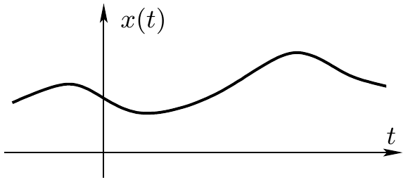
En general, consideramos que es el tiempo: x ( t ) x(t) x ( t )
Vamos a considerar dos tipos básicos de señales :
Continuas : la variable independiente es continua ⇒ \Rightarrow ⇒
Notación : x ( t ) \boxed{x(t)} x ( t ) t ∈ ℜ t\in\real t ∈ ℜ
Ejemplos: señal de voz con el tiempo, presión atmosférica con altitud.
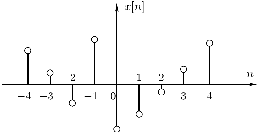
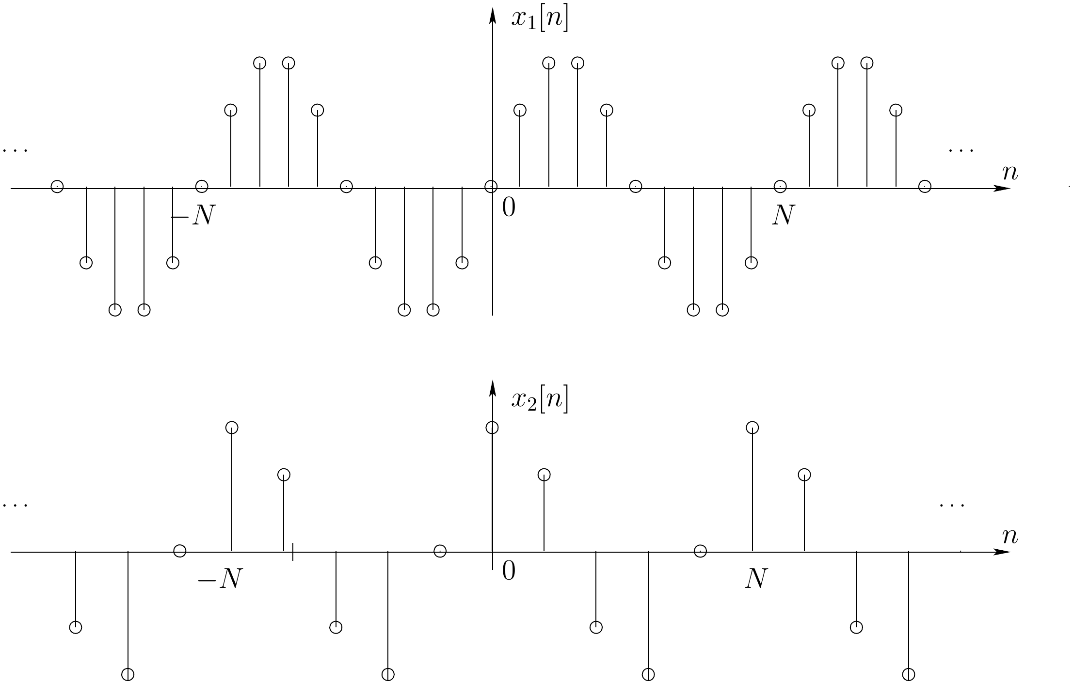
Discretas : la variable independiente sólo toma un conjunto discreto de valores. También se las llama secuencia discreta .
Notación : x [ n ] \boxed{x[n]} x [ n ] n ∈ Z n\in\Z n ∈ Z
Ejemplos: valor del IBEX-35 al final de cada sesión, muestreo de señales continuas (muestras equiespaciadas).
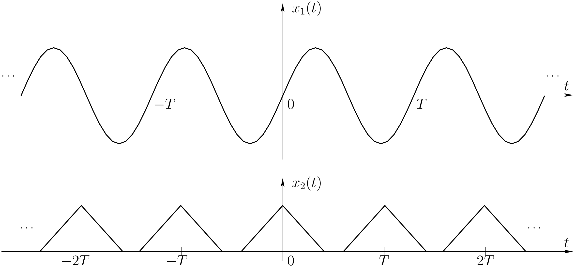
Se mostrarán las señales continuas y discretas de forma paralela, para irlas relacionando. En el capítulo de muestreo (7), veremos cómo se puede pasar de unas a otras, idealmente sin error.
Clases de señales ¶ Veremos a continuación distintos tipos de señales que tendrán importancia a lo largo de toda la asignatura.
Real e imaginaria : simetría respecto a la conjugación.
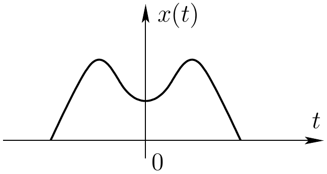
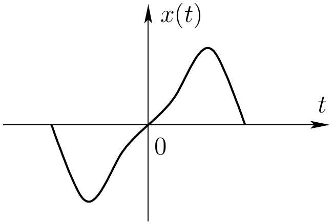
Par e impar : simetría respecto a la inversión en el tiempo. Se aplica a señales reales.
Par : simétrica respecto al eje de ordenadas.
x ( − t ) = x ( t ) , x(-t)=x(t), x ( − t ) = x ( t ) , x [ − n ] = x [ n ] . x[-n]=x[n]. x [ − n ] = x [ n ] . Impar : antisimétrica respecto al eje de ordenadas.
x ( − t ) = − x ( t ) , x(-t)=-x(t), x ( − t ) = − x ( t ) , x [ − n ] = − x [ n ] . x[-n]=-x[n]. x [ − n ] = − x [ n ] . En el origen, como x ( 0 ) = − x ( 0 ) x(0)=-x(0) x ( 0 ) = − x ( 0 )
Hermítica y antihermítica : Equivalente para señales complejas.
Toda señal se puede poner como suma de sus partes real e imaginaria, par e impar, hermítica y antihermítica:
x ( t ) = x r ( t ) + x i ( t ) = ℜ { x ( t ) } + ℑ { x ( t ) } . x(t)=x_r(t)+x_i(t)=\Re\{x(t)\}+\Im\{x(t)\}. x ( t ) = x r ( t ) + x i ( t ) = ℜ { x ( t )} + ℑ { x ( t )} . x ( t ) = x e ( t ) + x o ( t ) = E v { x ( t ) } + O d { x ( t ) } , x ( t ) ∈ ℜ . x(t)=x_e(t)+x_o(t)=\mathcal{Ev}\{x(t)\}+\mathcal{Od}\{x(t)\},\quad x(t)\in\real. x ( t ) = x e ( t ) + x o ( t ) = E v { x ( t )} + O d { x ( t )} , x ( t ) ∈ ℜ. x ( t ) = x h ( t ) + x a ( t ) . x(t)=x_h(t)+x_a(t). x ( t ) = x h ( t ) + x a ( t ) . Las expresiones para el caso discreto son equivalentes.
Cálculo de la parte par e impar de una señal:
{ x ( t ) = x e ( t ) + x o ( t ) , x ( − t ) = x e ( − t ) + x o ( − t ) = x e ( t ) − x o ( t ) \begin{cases}x(t)=x_e(t)+x_o(t),\\x(-t)=x_e(-t)+x_o(-t)=x_e(t)-x_o(t)\end{cases} { x ( t ) = x e ( t ) + x o ( t ) , x ( − t ) = x e ( − t ) + x o ( − t ) = x e ( t ) − x o ( t ) Parte par e impar de una señal:
{ x e ( t ) = 1 2 [ x ( t ) + x ( − t ) ] , x o ( t ) = 1 2 [ x ( t ) − x ( − t ) ] \begin{cases}x_e(t)=\frac{1}{2}\left[x(t)+x(-t)\right],\\x_o(t)=\frac{1}{2}\left[x(t)-x(-t)\right]\end{cases} { x e ( t ) = 2 1 [ x ( t ) + x ( − t ) ] , x o ( t ) = 2 1 [ x ( t ) − x ( − t ) ] Se cumple:
x e ( 0 ) = x ( 0 ) , x e [ 0 ] = x [ 0 ] . x_e(0)=x(0),\qquad x_e[0]=x[0]. x e ( 0 ) = x ( 0 ) , x e [ 0 ] = x [ 0 ] . x o ( 0 ) = 0 , x o [ 0 ] = 0. x_o(0)=0,\qquad x_o[0]=0. x o ( 0 ) = 0 , x o [ 0 ] = 0. Parte real e imaginaria:
{ x r ( t ) = 1 2 [ x ( t ) + x ∗ ( t ) ] , x i ( t ) = 1 2 [ x ( t ) − x ∗ ( t ) ] \begin{cases}x_r(t)=\frac{1}{2}\left[x(t)+x^*(t)\right],\\x_i(t)=\frac{1}{2}\left[x(t)-x^*(t)\right]\end{cases} { x r ( t ) = 2 1 [ x ( t ) + x ∗ ( t ) ] , x i ( t ) = 2 1 [ x ( t ) − x ∗ ( t ) ] Parte hermítica y antihermítica:
{ x h ( t ) = 1 2 [ x ( t ) + x ∗ ( − t ) ] , x a ( t ) = 1 2 [ x ( t ) − x ∗ ( − t ) ] \begin{cases} x_h(t)=\frac{1}{2}\left[x(t)+x^*(-t)\right],\\x_a(t)=\frac{1}{2}\left[x(t)-x^*(-t)\right]\end{cases} { x h ( t ) = 2 1 [ x ( t ) + x ∗ ( − t ) ] , x a ( t ) = 2 1 [ x ( t ) − x ∗ ( − t ) ] Para el caso discreto las expresiones son equivalentes.
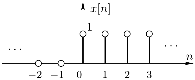
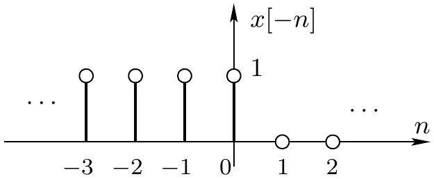
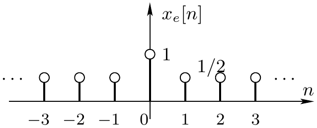
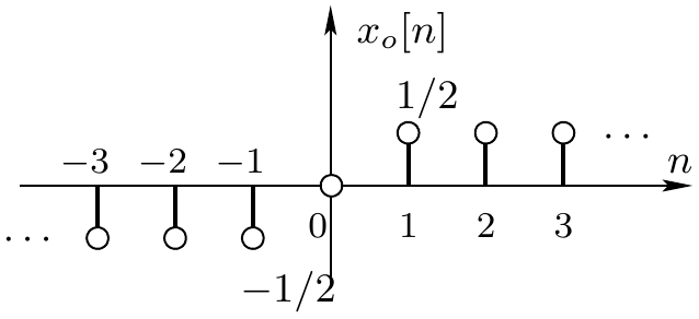
Ejemplo : Cálculo de la parte par e impar de una señal:
x [ n ] = { 1 , n ≥ 0 , 0 , n < 0 x[n]=\begin{cases} 1, & n\ge 0,\\0, & n<0\end{cases} x [ n ] = { 1 , 0 , n ≥ 0 , n < 0
x [ − n ] = { 1 , n ≤ 0 , 0 , n > 0 x[-n]=\begin{cases} 1, & n\le 0,\\0, & n>0\end{cases} x [ − n ] = { 1 , 0 , n ≤ 0 , n > 0
x e [ n ] = { 1 / 2 , n < 0 , 1 , n = 0 , 1 / 2 , n > 0 x_e[n]=\begin{cases} 1/2, & n<0,\\1, & n=0,\\1/2, & n>0\end{cases} x e [ n ] = ⎩ ⎨ ⎧ 1/2 , 1 , 1/2 , n < 0 , n = 0 , n > 0
x o [ n ] = { − 1 / 2 , n < 0 , 0 , n = 0 , 1 / 2 , n > 0 x_o[n]=\begin{cases} -1/2, & n<0,\\0, & n=0,\\1/2, & n>0\end{cases} x o [ n ] = ⎩ ⎨ ⎧ − 1/2 , 0 , 1/2 , n < 0 , n = 0 , n > 0
A continuación veremos otros tipos de señales: periódicas, de energía y de potencia.
Señales periódicas ¶ Dada su importancia las vemos aparte.
∃ T ∈ ℜ + / x ( t ) = x ( t + T ) , ∀ t ∈ ℜ . \exists\ T\in\real^+ /\quad \boxed{x(t)=x(t+T)},\quad \forall t\in\real. ∃ T ∈ ℜ + / x ( t ) = x ( t + T ) , ∀ t ∈ ℜ. T T T periodo de la señal.
Ejemplos :
Si x ( t ) x(t) x ( t ) T T T m T , m ∈ N mT,\ m\in\N m T , m ∈ N
T 0 T_0 T 0 periodo fundamental de la señal. Valor más pequeño de T T T
x ( t ) = x ( t + T 0 ) . x(t)=x(t+T_0). x ( t ) = x ( t + T 0 ) . Si x ( t ) x(t) x ( t ) T 0 T_0 T 0 T T T
Ejemplos:
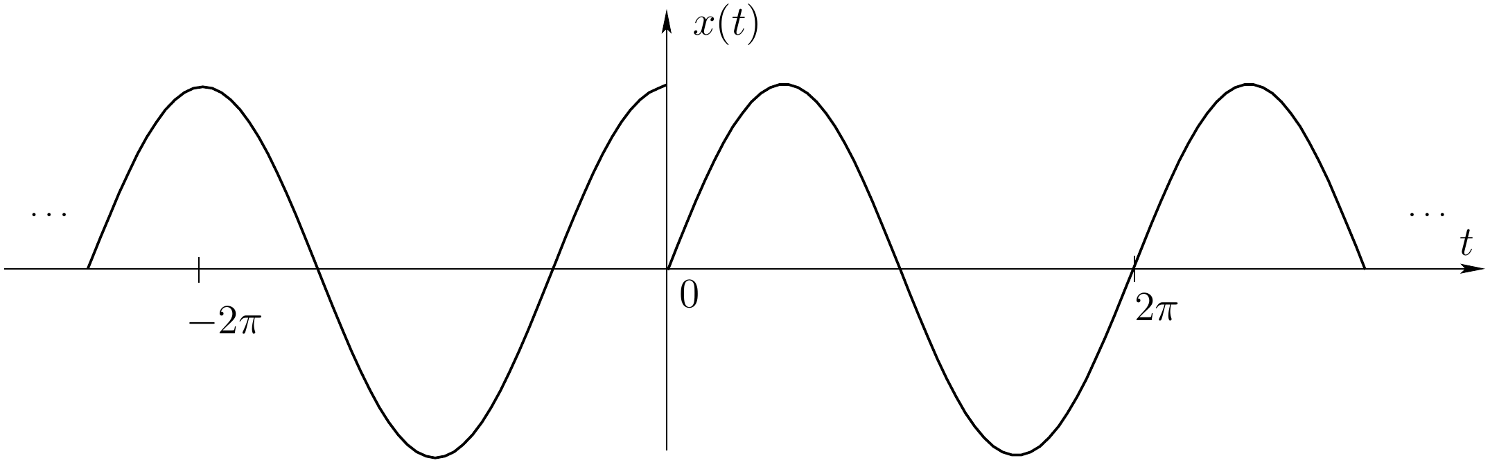
x ( t ) = { cos ( t ) , t < 0 , sin ( t ) , t ≥ 0 x(t)=\begin{cases} \cos(t), & t<0,\\ \sin(t), & t\ge 0\end{cases} x ( t ) = { cos ( t ) , sin ( t ) , t < 0 , t ≥ 0 Se cumple que cos ( t ) = cos ( t + 2 π ) \cos(t)=\cos(t+2\pi) cos ( t ) = cos ( t + 2 π ) t < − 2 π t<-2\pi t < − 2 π sin ( t ) = sin ( t + 2 π ) \sin(t)=\sin(t+2\pi) sin ( t ) = sin ( t + 2 π ) t ≥ 0 t\ge0 t ≥ 0 x ( t ) = x ( t + 2 π ) , ∀ t x(t)=x(t+2\pi),\ \forall t x ( t ) = x ( t + 2 π ) , ∀ t
Estudiar el caso:
x ( t ) = { cos ( t ) , t < 0 , cos ( − t ) , t ≥ 0 x(t)=\begin{cases} \cos(t), & t<0,\\ \cos(-t), & t\ge 0 \end{cases} x ( t ) = { cos ( t ) , cos ( − t ) , t < 0 , t ≥ 0 ∃ N ∈ N / x [ n ] = x [ n + N ] , ∀ n ∈ Z . \exists\ N\in\N /\quad \boxed{x[n]=x[n+N]},\quad \forall n\in\Z. ∃ N ∈ N / x [ n ] = x [ n + N ] , ∀ n ∈ Z . N N N periodo de la señal.
Ejemplos :
Si x [ n ] x[n] x [ n ] N N N m N , m ∈ N mN,\ m\in\N m N , m ∈ N
N 0 N_0 N 0 periodo fundamental de la secuencia discreta. Valor más pequeño de N N N
x [ n ] = x [ n + N 0 ] . x[n]=x[n+N_0]. x [ n ] = x [ n + N 0 ] . Si x [ n ] x[n] x [ n ] N 0 = 1 N_0=1 N 0 = 1
Parámetros de interés ¶ Vemos algunos parámetros de interés de las señales, tanto continuas como discretas.
Valor medio :
En el intervalo t 1 ≤ t ≤ t 2 t_1\le t\le t_2 t 1 ≤ t ≤ t 2
x ˉ = Δ 1 t 2 − t 1 ∫ t 1 t 2 x ( t ) d t . \bar{x}\overset{\Delta}{=}\frac{1}{t_2-t_1}\int_{t_1}^{t_2} x(t)dt. x ˉ = Δ t 2 − t 1 1 ∫ t 1 t 2 x ( t ) d t . Para un intervalo simétrico, − T ≤ t ≤ T -T\le t\le T − T ≤ t ≤ T
x ˉ = Δ 1 2 T ∫ − T T x ( t ) d t . \bar{x}\overset{\Delta}{=}\frac{1}{2T}\int_{-T}^T x(t)dt. x ˉ = Δ 2 T 1 ∫ − T T x ( t ) d t . En el intervalo n 1 ≤ n ≤ n 2 n_1\le n\le n_2 n 1 ≤ n ≤ n 2
x ˉ = Δ 1 n 2 − n 1 + 1 ∑ n = n 1 n 2 x [ n ] . \bar{x}\overset{\Delta}{=}\frac{1}{n_2-n_1+1}\sum\limits_{n=n_1}^{n_2} x[n]. x ˉ = Δ n 2 − n 1 + 1 1 n = n 1 ∑ n 2 x [ n ] . Para un intervalo simétrico, − N ≤ n ≤ N -N\le n\le N − N ≤ n ≤ N
x ˉ = Δ 1 2 N + 1 ∑ n = − N N x [ n ] . \bar{x}\overset{\Delta}{=}\frac{1}{2N+1}\sum\limits_{n=-N}^N x[n]. x ˉ = Δ 2 N + 1 1 n = − N ∑ N x [ n ] . Valor de pico :
x p = Δ max { ∣ x ( t ) ∣ , t ∈ ℜ } . x_p\overset{\Delta}{=}\max\{|x(t)|,\ t\in\real\}. x p = Δ max { ∣ x ( t ) ∣ , t ∈ ℜ } . x p = Δ max { ∣ x [ n ] ∣ , n ∈ Z } . x_p\overset{\Delta}{=}\max\{|x[n]|,\ n\in\Z\}. x p = Δ max { ∣ x [ n ] ∣ , n ∈ Z } . Potencia instantánea :
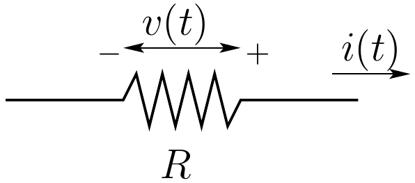
Así, por ejemplo, para una resistencia, la potencia instantánea es:
p ( t ) = v ( t ) i ( t ) = 1 R v 2 ( t ) = R i 2 ( t ) . p(t)=v(t)i(t)=\frac{1}{R}v^2(t)=Ri^2(t). p ( t ) = v ( t ) i ( t ) = R 1 v 2 ( t ) = R i 2 ( t ) . Vemos que es proporcional a la señal al cuadrado. En otros ejemplos ocurre lo mismo.
P i ( t ) = Δ ∣ x ( t ) ∣ 2 . P_i(t)\overset{\Delta}{=}|x(t)|^2. P i ( t ) = Δ ∣ x ( t ) ∣ 2 . P i [ n ] = Δ ∣ x [ n ] ∣ 2 . P_i[n]\overset{\Delta}{=}|x[n]|^2. P i [ n ] = Δ ∣ x [ n ] ∣ 2 . Energía : suma (integral) de la potencia instantánea.
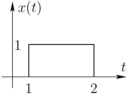
Hay señales para las que esta integral (sumatorio) no converge, como por ejemplo:
x 1 ( t ) = 1 t , x 2 ( t ) = C . x_1(t)=\frac{1}{\sqrt{t}},\qquad x_2(t)=C. x 1 ( t ) = t 1 , x 2 ( t ) = C . x 1 [ n ] = 1 n , x 2 [ n ] = C . x_1[n]=\frac{1}{\sqrt{n}},\qquad x_2[n]=C. x 1 [ n ] = n 1 , x 2 [ n ] = C . En estos casos, E ∞ = ∞ . E_\infty=\infty. E ∞ = ∞.
Por ello, nos va a interesar otra medida relacionada, que es la potencia media.
Potencia media : valor medio de la potencia instantánea.
En general, la potencia media viene dada por:
P ∞ = Δ lim T → ∞ 1 T ∫ − T / 2 T / 2 ∣ x ( t ) ∣ 2 d t = lim T → ∞ 1 2 T ∫ − T T ∣ x ( t ) ∣ 2 d t . P_\infty\overset{\Delta}{=}\lim_{T\to\infty}\frac{1}{T}\int_{-T/2}^{T/2} |x(t)|^2dt=\lim_{T\to\infty}\frac{1}{2T}\int_{-T}^{T} |x(t)|^2dt. P ∞ = Δ T → ∞ lim T 1 ∫ − T /2 T /2 ∣ x ( t ) ∣ 2 d t = T → ∞ lim 2 T 1 ∫ − T T ∣ x ( t ) ∣ 2 d t . P ∞ = Δ lim N → ∞ 1 2 N + 1 ∑ n = − N N ∣ x [ n ] ∣ 2 . P_\infty\overset{\Delta}{=}\lim_{N\to\infty}\frac{1}{2N+1}\sum\limits_{n=-N}^{N} |x[n]|^2. P ∞ = Δ N → ∞ lim 2 N + 1 1 n = − N ∑ N ∣ x [ n ] ∣ 2 . En el caso particular de señales periódicas , también son aplicables las siguientes expresiones:
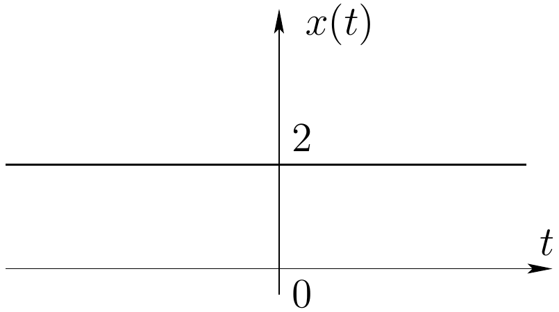
P ∞ = Δ 1 T ∫ < T > ∣ x ( t ) ∣ 2 d t . P_\infty\overset{\Delta}{=}\frac{1}{T}\int_{<T>} |x(t)|^2dt. P ∞ = Δ T 1 ∫ < T > ∣ x ( t ) ∣ 2 d t . P ∞ = Δ 1 N ∑ n ∈ < N > ∣ x [ n ] ∣ 2 . P_\infty\overset{\Delta}{=}\frac{1}{N}\sum\limits_{n\in<N>} |x[n]|^2. P ∞ = Δ N 1 n ∈< N > ∑ ∣ x [ n ] ∣ 2 . Ejemplo : x ( t ) = 2. x(t)=2. x ( t ) = 2.
P i ( t ) = ∣ x ( t ) ∣ 2 = 4. P_i(t)=|x(t)|^2=4. P i ( t ) = ∣ x ( t ) ∣ 2 = 4. E ∞ = ∫ − ∞ ∞ ∣ x ( t ) ∣ 2 d t = ∫ − ∞ ∞ 4 d t = ∞ . E_\infty=\int_{-\infty}^\infty |x(t)|^2 dt=\int_{-\infty}^\infty 4 dt=\infty. E ∞ = ∫ − ∞ ∞ ∣ x ( t ) ∣ 2 d t = ∫ − ∞ ∞ 4 d t = ∞. P ∞ = lim T → ∞ 1 T ∫ − T / 2 T / 2 P i ( t ) d t = lim T → ∞ 4 T T = 4. P_\infty=\lim_{T\to\infty}\frac{1}{T}\int_{-T/2}^{T/2} P_i(t) dt=\lim_{T\to\infty}\frac{4T}{T}=4. P ∞ = T → ∞ lim T 1 ∫ − T /2 T /2 P i ( t ) d t = T → ∞ lim T 4 T = 4. Señales de energía y de potencia ¶ Según las definiciones de energía y de potencia de una señal, se puede hablar de tres clases de señales:
0 < E ∞ < ∞ . 0<E_\infty<\infty. 0 < E ∞ < ∞. Tienen P ∞ = 0 P_\infty=0 P ∞ = 0
P ∞ = lim T → ∞ 1 2 T ∫ − T T ∣ x ( t ) ∣ 2 d t = lim T → ∞ E T 2 T = 0. P_\infty=\lim_{T\to\infty}\frac{1}{2T}\int_{-T}^{T} |x(t)|^2dt=\lim_{T\to\infty}\frac{E_T}{2T}=0. P ∞ = T → ∞ lim 2 T 1 ∫ − T T ∣ x ( t ) ∣ 2 d t = T → ∞ lim 2 T E T = 0. P ∞ = lim N → ∞ 1 2 N + 1 ∑ n = − N N ∣ x [ n ] ∣ 2 = lim N → ∞ E N 2 N + 1 = 0. P_\infty=\lim_{N\to\infty}\frac{1}{2N+1}\sum\limits_{n=-N}^{N} |x[n]|^2=\lim_{N\to\infty}\frac{E_N}{2N+1}=0. P ∞ = N → ∞ lim 2 N + 1 1 n = − N ∑ N ∣ x [ n ] ∣ 2 = N → ∞ lim 2 N + 1 E N = 0. Ejemplo :
E ∞ = 1 ⇒ P ∞ = 0. E_\infty=1 \Rightarrow P_\infty=0. E ∞ = 1 ⇒ P ∞ = 0. 0 < P ∞ < ∞ ⇒ E ∞ = ∞ . 0<P_\infty<\infty \quad \Rightarrow \quad E_\infty=\infty. 0 < P ∞ < ∞ ⇒ E ∞ = ∞. Dado que tienen P ∞ > 0 P_\infty>0 P ∞ > 0 E ∞ = ∞ E_\infty=\infty E ∞ = ∞
Ejemplos :
x 1 ( t ) = 2. x_1(t)=2. x 1 ( t ) = 2. x 2 ( t ) x_2(t) x 2 ( t ) x p x_p x p
Ejemplo :
x ( t ) = t . x(t)=t. x ( t ) = t .
E ∞ = lim T → ∞ ∫ − T T ∣ t ∣ 2 d t = lim T → ∞ ∫ − T T t 2 d t = lim T → ∞ t 3 ∣ − T T 3 = lim T → ∞ 2 T 3 3 = ∞ . E_\infty=\lim_{T\to\infty}\int_{-T}^{T}|t|^2 dt=\lim_{T\to\infty}\int_{-T}^{T}t^2 dt=\lim_{T\to\infty}\frac{\left.t^3\right|_{-T}^{T}}{3}=
\lim_{T\to\infty}\frac{2T^3}{3}=\infty. E ∞ = T → ∞ lim ∫ − T T ∣ t ∣ 2 d t = T → ∞ lim ∫ − T T t 2 d t = T → ∞ lim 3 t 3 ∣ ∣ − T T = T → ∞ lim 3 2 T 3 = ∞. P ∞ = lim T → ∞ 1 2 T ∫ − T T ∣ t ∣ 2 d t = lim T → ∞ E T 2 T = lim T → ∞ 2 T 3 6 T = ∞ . P_\infty=\lim_{T\to\infty}\frac{1}{2T}\int_{-T}^{T}|t|^2 dt=\lim_{T\to\infty}\frac{E_T}{2T}=\lim_{T\to\infty}\frac{2T^3}{6T}=\infty. P ∞ = T → ∞ lim 2 T 1 ∫ − T T ∣ t ∣ 2 d t = T → ∞ lim 2 T E T = T → ∞ lim 6 T 2 T 3 = ∞.