Visualize

Data visualization

# load sample data
data4D = img2float(cells3d())
data = data4D[:, 1, :, :] # load the nuclei channel

Display 2D images

Function to quickly display 2D images

source

plot_image

 plot_image (values)

*Plot a 2D image using Matplotlib. The function assumes that ‘values’ is a 2D array representing an image, typically in grayscale.

Parameters: values (numpy.ndarray): A 2D array of pixel values representing the image.

Returns: None*

# Example usage:
plot_image(data[35])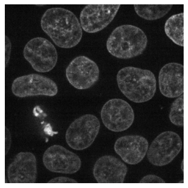

Display Multichannel images

Function to display RGB and multichannel images

source

show_multichannel

 show_multichannel (img, ax=None, figsize=None, title=None, max_slices=3,
                    ctx=None, cmap=None, norm=None, aspect=None,
                    interpolation=None, alpha=None, vmin=None, vmax=None,
                    origin=None, extent=None, interpolation_stage=None,
                    filternorm=True, filterrad=4.0, resample=None,
                    url=None, data=None, **kwargs)

Show multi-channel CYX image.

Display 3D images

Function to display 3D images

source

mosaic_image_3d

 mosaic_image_3d (t:(<class'numpy.ndarray'>,<class'torch.Tensor'>),
                  axis:int=0, figsize:tuple=(15, 15), cmap:str='gray',
                  nrow:int=10, alpha=1.0, return_grid=False,
                  add_to_existing=False, **kwargs)

Plots 2D slices of a 3D image alongside a prior specified axis. Args: t: a 3D numpy.ndarray or torch.Tensor axis: axis to split 3D array to 2D images figsize, cmap: passed to plt.imshow nrow: passed to torchvision.utils.make_grid return_grid: Whether the grid should be returned for further processing or if the plot should be displayed. add_to_existing: if set to true, no new figure will be created. Used for mask overlays

source

show_images_grid

 show_images_grid (images, ax=None, ncols=10, figsize=None, title=None,
                   spacing=0.02, max_slices=3, ctx=None, cmap=None,
                   norm=None, aspect=None, interpolation=None, alpha=None,
                   vmin=None, vmax=None, origin=None, extent=None,
                   interpolation_stage=None, filternorm=True,
                   filterrad=4.0, resample=None, url=None, data=None,
                   **kwargs)

*Show a list of images arranged in a grid.

Parameters: - images: list of images to display. - ncols (int): number of columns in the grid. - figsize (tuple, optional): figure size in inches. - title (list, optional): list of titles corresponding to each image. - spacing (float, optional): spacing between subplots. - ctx: additional context passed to the plt.Axes.imshow function. - **kwargs: additional keyword arguments passed to plt.Axes.imshow.

Returns: - axes: matplotlib axes containing the grid of images.*

mosaic_image_3d(torch_from_numpy(data), figsize=None)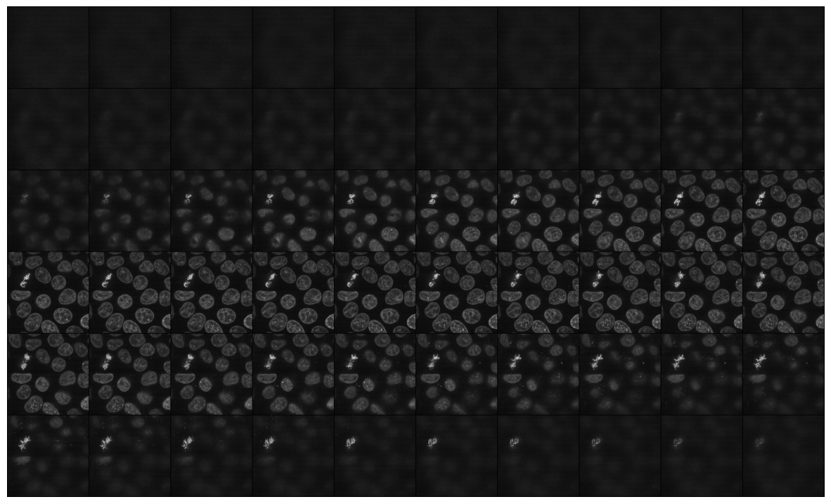

show_images_grid(data, cmap='gray');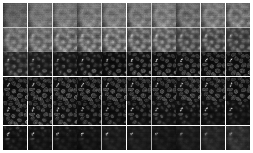

Show slices

source

show_plane

 show_plane (ax, plane, cmap='gray', title=None, lines=None,
             linestyle='--', linecolor='white')

*Display a slice of the image tensor on a given axis with optional dashed lines.

Parameters: ax (matplotlib.axes._subplots.AxesSubplot): The axis object to display the slice on. plane (numpy.ndarray): A 2D numpy array representing the slice of the image tensor. cmap (str, optional): Colormap to use for displaying the image. Defaults to “gray”. title (str, optional): Title for the plot. Defaults to None. dashed_lines (list, optional): A list of indices where dashed lines should be drawn on the plane.*

source

visualize_slices

 visualize_slices (data, planes=None, showlines=True, **kwargs)

*Visualize slices of a 3D image tensor along its planes, rows, and columns.

Parameters: data (numpy.ndarray): A 3D numpy array representing the image tensor. planes (tuple): A tuple containing the indices of the planes to visualize. If None, defaults to middle slices.*

visualize_slices(data, showlines=False)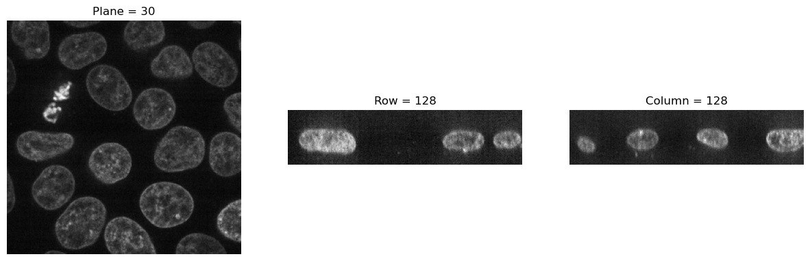

visualize_slices(data, (25,100,150), linestyle=':')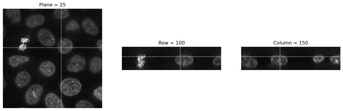

source

slice_explorer

 slice_explorer (data, order='CZYX', **kwargs)

*Visualizes the provided data using Plotly’s interactive imshow function with animation support.

Args: data (np.array or pd.DataFrame): The data to be visualized, typically a 2D array representing an image sequence. order (str): The order of dimensions in the data (e.g., ‘CZYX’).

Returns: None: Displays the plot directly.*

slice_explorer(data4D, order='ZCYX', title='Cells 3D')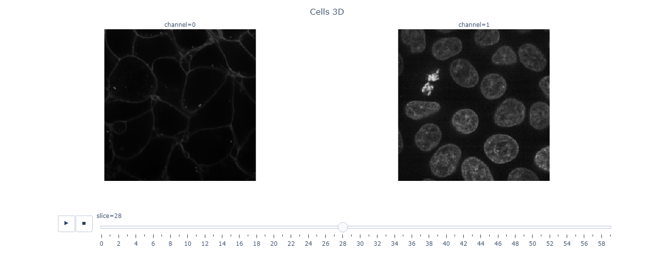

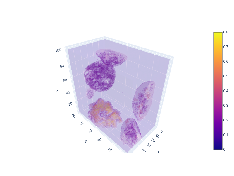
source

plot_volume

 plot_volume (values, opacity=0.1, min=0.1, max=0.8, surface_count=5,
              width=800, height=600)

*Plot a 3D volume using Plotly. The function assumes that ‘values’ is a 3D array representing the volume data.

Parameters: values (numpy.ndarray): A 3D array of pixel values representing the volume. opacity (float, optional): Opacity level for the surfaces in the volume plot. Defaults to 0.1. min (float, optional): Minimum threshold multiplier for the visualization. Defaults to 0.1. max (float, optional): Maximum threshold multiplier for the visualization. Defaults to 0.8. surface_count (int, optional): Number of surfaces to display in the volume plot. Defaults to 5. width (int, optional): Width of the plotted figure. Defaults to 800. height (int, optional): Height of the plotted figure. Defaults to 600.

Returns: None*

plot_volume(data[:, 50:150, 50:150])

Unable to display output for mime type(s): application/vnd.plotly.v1+json